Schlagwort-Archive: Groovy

Window Functions in RapidMiner

(English version)

Window-Funktionen in RapidMiner

Richtige Datenbankserver wie PostgreSQL haben seit geraumer Zeit den SQL-99-Standard umgesetzt, der unter anderem Window Functions beschreibt.

Mit Window Functions lassen sich gruppenbezogene Statistiken und Kennzahlen berechnen, ohne die Ergebnismenge zu gruppieren. (Dies ist der Unterschied zur klassischen Aggregierung mit GROUP BY.) Es gibt eine Menge Anwendungsbeispiele: es lassen sich laufende Summen, gleitende Mittelwerte, Anteile innerhalb der Gruppe, gruppenweise Minima oder Maxima und noch viele andere Dinge berechnen. Manche Leute meinen, daß mit Window Functions eine neue Ära für SQL begonnen hat, und ich neige dazu, ihnen zuzustimmen.

RapidMiner hat bislang keine Window Functions eingebaut. Erfahrene Data Scientists, die Bedarf an dieser Funktionalität hatten, haben diese mit verschiedenen Operatoren (Loops, gruppenweise Aggregation und Join usw.) selbst nachbauen können, aber das ist alles andere als trivial.

Um die Funktionalität für einen größeren Benutzerkreis zu öffnen und gleichzeitig eine wiederverwendbare Implementierung zu schaffen, habe ich das Projekt rapidminer-windowfunctions ins Leben gerufen und eine erste funktionierende Implementierung hochgeladen.

Alle im RapidMiner-Operator „Aggregate“ eingebauten Aggregationsfunktionen lassen sich verwenden: sum, average, minimum, maximum usw. Zusätzlich sind die Funktionen row_number, rank und dense_rank verfügbar.

Im Projektordner sind der eigentliche Prozess und aktuell drei Beispielprozesse enthalten, um gleich verschiedene Anwendungsmöglichkeiten testen zu können.

Golf-Datensatz: Gruppenmittelwert der Temperatur und Rang innerhalb der Gruppe für Luftfeuchtigkeit
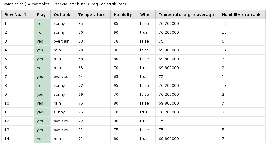
  • Golf: Der berühmte Golf-Dataset wird aus dem mitgelieferten Beispiel-Repository geladen. Für jede Gruppe basierend auf dem „Outlook“-Attribut wird die Durchschnittstemperatur berechnet und als Attribut hinzugefügt. Ein zweites neues Attribut enthält den Rang des Datensatzes bei Sortierung nach dem Wert der Luftfeuchtigkeit. Gleiche Werte erhalten den gleichen Rang.
  • Iris: Ein weiterer Standard-Dataset, Iris, wird geladen, und es wird pro Spezies der Durchschnittswert fürs Attribut „a3“ berechnet. Dieser Mittelwert wird dann genutzt, um Exemplare herauszufiltern, die mehr als 10 % vom Gruppenmittelwert entfernt sind.
  • Deals: Der mitgelieferte Dataset „Deals“ wird geladen. In jeder Kundengruppe aus Geschlecht und Zahlungsmethode werden die drei ältesten Kunden gesucht, die anderen werden herausgefiltert.

Das zeigt schon die Bandbreite der Möglichkeiten, die Window Functions bieten. Die Möglichkeit, sie leicht einzusetzen und Indikatoren sowie Kennzahlen wie „Transaktionszähler des Kunden im Monat“, „Anteil des Produkts an der Monatssumme“ und ähnliche erzeugen zu können, wird viele Prozesse vereinfachen, oder neue Möglichkeiten eröffnen.

Implementierung

Nach einigen Prüfungen, z. B. ob die benötigten Makros gesetzt sind, werden neue Attribute zur Gruppierung und Identifizierung von Examples angelegt. Das zusammengesetzte Gruppierungsattribut wird dabei aus den Werten der als groupFields angegebenen Attribute generiert. Das Identifizerungs-Attribut muß mit einem Groovy-Skript generiert werden, da Generate Id mit vielen Datensätzen nicht funktionieren würde. (Generate Id funktioniert nicht, wenn der Datensatz bereits ein Attribut mit der Rolle id enthält.)

Die drei Spezialfunktionen, die in Aggregate nicht enthalten sind, werden gesondert behandelt. Die Untergruppen werden nach dem ausgewählten Attribut sortiert und der Datensatzzähler bzw. die Rangfolge berechnet.

Die Standard-Aggregierungsfunktionen von RapidMiner werden einfach auf jede Subgruppe angewendet, dabei entsteht jeweils eine gruppierte Zeile. Diese wird wieder mit den Originaldaten gejoint.

Einschränkungen

Gegenüber dem SQL-Standard und der in Datenbanken implementierten Funktionalität fehlt noch einiges. Z. B. erlauben Datenbanken bei Funktionen wie SUM die Angabe eines Sortierkriteriums und berechnen dann eine kumulierte Summe für jede Zeile, statt die gleiche Summe wiederholt auszugeben.

Der Prozess ist auch recht langsam, wenn viele Gruppen existieren. Dies ergibt eine große Anzahl von Filterungen in der Schleife. Bei den speziellen Rang- und Zählerfunktionen ist das Problem besonders ausgeprägt, da in jedem Durchlauf ein Groovy-Interpreter gestartet wird, was erhebliche Zeit kostet.

Das Konzept von Window-Definitionen geht in SQL-Datenbanken über Selektion von Gruppen hinaus. Z. B. kann man in SQL auf den vorherigen oder nächsten Datensatz zugreifen (LAG bzw. LEAD), ein fixes Fenster von X Zeilen definieren, und in den Daten „nach vorne“ schauen. Diese Dinge sind gegenwärtig nicht im Prozess eingebaut.

Mögliche Erweiterungen

Es spricht nichts dagegen, einige von den in SQL zur Verfügung stehenden Funktionen wie percent_rank, ntile oder first/last_value einzubauen. Dies wird bei Bedarf sicher passieren.

Die Funktionalität, über ORDER BY das Verhalten der Aggregierungsfunktionen zu ändern (z. B. für kumulierte Summen), erscheint mit RapidMiner-Mitteln nicht einfach. Allerdings ließe sich die kumulierte Summe leicht mit einem weiteren Groovy-Skript implementieren.

Bezugsquelle

Das Projekt kann auf Github heruntergeladen oder ausgecheckt werden. Es enthält Dokumentation und Beispielprozesse. Die Lizenz ist Apache 2.0, somit sind Einsatz und Weiterentwicklung uneingeschränkt möglich. Es ist also ein klassisches Open-Source-Projekt, das von der Beteiligung und Weiterentwicklung durch die Community leben soll.

Window functions in RapidMiner

For powerful database software like PostgreSQL the SQL-99 standard has been implemented for a long time. Window functions are an important part of SQL-99.

Window functions are used for calculating groupwise statistics and measures without actually grouping the result. (This is the difference between Window functions and the well-known aggregation with GROUP BY.) There are many applications: running sums, moving averages, ratios inside a group, groupwise minimum and maximum and so on. Some people consider the introduction of Window functions the beginning of a new era for SQL. I agree with this quite strongly.

RapidMiner doesn’t offer Window functions, yet. Experienced data scientists were able to build this functionality when they had to, using loops, aggregation and join, but these processes are not easy to create and debug.

My goal is to open this functionality for a larger group of potential users and to create a reusable implementation. So I started the rapidminer-windowfunctions project and uploaded the first working version.

All functions built into RapidMiner’s Aggregate operator can be used: sum, average, minimum, maximum etc. Additional functions are row_number, rank and dense_rank.

The project ships with the actual process and a number of example processes. These demonstrate different applications of Window functions on public datasets available in RapidMiner Studio.

Golf dataset with groupwise temperature average and rank by humidity
  • Golf: The process loads the well-known Golf dataset from the Samples repository. For each group defined by the attribute “Outlook”, the average temperature gets calculated. A second attribute ranks the examples by the attribute “Humidity”. Identical values get the same rank.

  • Iris: This is another standard dataset, available from RapidMiner’s Samples repository. The process calculates the average value for the attribute “a3”. This group average is used to filter out examples which differ from the average by more than 10 %.

  • Deals: Another data set built into RapidMiner. This process considers all combinations of Gender and Payment Method as groups and ranks the customers based on their age. Only the 3 oldest customers per group are retained.

This is just a small sample of all the functionality available with Window Functions. Being able to use them easily for building indicators and measures like “transaction counter per customer and month” or “the product’s contribution percentage” will open new possibilities for modelling or reporting.

Implementation

The process checks a few preconditions, for example required parameter macros. It creates new attributes for grouping and identifying examples. The grouping attribute is built from all values given in the groupFields parameter. The identifying attribute needs to be generated in a Groovy script, as Generate Id would fail on too many real-world datasets. (It doesn’t work when the dataset already has an attribute with the role id.)

The three special functions not available in Aggregate are implemented with Groovy scripts. The process sorts the subgroups by the selected attributes and calculates the record counter or the rank.

The implementation of the standard aggregations is simpler: each subgroup is aggregated and the result is joined with the original data.

Limitations

Some functionality is missing compared to the SQL standard and to database systems. For example, in SQL databases, you can use ORDER BY in the window function to specify an ordering and calculate cumulative sums for each row instead of a groupwise sum.

The process is quite slow if many groups exist in the dataset. Having many groups results in a large number of filters in the loop. The performance is especially bad with the special ranking and counter functions because they start a Groovy interpreter in each iteration, which takes a lot of time compared to other operators.

The concept of window definition in SQL databases covers more than just the selection of groups. For example, you can access the previous and next records (LAG and LEAD), define a fixed window of N rows, and look forward in the data. These things are not available in the current version of the process.

Possible extensions

It’s entirely possible to implement more SQL standard functions like percent_rank, ntile and first/last_value. This will happen for sure when there’s a need.

It seems to be hard to change the behaviour of aggregation functions using ORDER BY (e. g. for cumulative sums) with RapidMiner means. However, special cases like the cumulative sum could be implemented with another Groovy script.

Getting the process

You can download the process or check it out on Github. The project also contains documentation and example processes. The license is Apache 2.0, so there are no restrictions on usage or further development. It is intended to become an Open Source project with the participation of and further development by the community.

Generic Joins in RapidMiner

Allgemeine Joins in RapidMiner

(English version)

Der letzte Beitrag hat sich mit der Verbesserung von geographischen Joins in RapidMiner beschäftigt. Tatsächlich kann die beschriebene Methode aber auf alle Arten von Joins angewendet werden, die nicht nur für einen kleinen Nutzerkreis interessant sind.

Der eingebaute Join-Operator in RapidMiner erlaubt nur „ist gleich“-Vergleiche. In der Praxis sind aber auch andere Operationen nützlich: z. B. reguläre Ausdrücke, oder „kleiner gleich“.

Der Beispielprozess nutzt generierte Testdaten und wendet eine Liste von regulären Ausdrücken auf sie an. Wie schon bei den geographischen Joins wird dafür ein Scripting-Operator mit einem Groovy-Skript verwendet.

Das Skript muß wie gehabt ziemlich viel Datenverwaltung betreiben, um die resultierende Tabelle aus den beiden Eingangs-Tabelle zu bauen. Bei der Erstellung des Skripts war wichtig, daß es möglichst allgemein verwendbar ist. Das ist in Groovy mit Hilfe der Closure-Syntax möglich: die Join-Funktion wird am Anfang des Skripts als eine Art Konfigurationsvariable festgelegt. Somit sind im Skript nur drei Dinge festzulegen: die beiden Join-Attribute und der Ausdruck, der auf sie anzuwenden ist.

In diesem Beispiel:

es1AttName = "Person";
es2AttName = "regexp";

def joinFunc = { e1, e2 ->
    e1.matches(e2)
}

Die beiden Attributsvariablen aus Example Set 1 und 2 werden am Anfang angegeben. Hier müssen die Attributnamen exakt (inkl. Groß- und Kleinschreibung) angegeben werden.

Die Closure joinFunc nimmt zwei Parameter (e1 und e2) entgegen, das sind die Werte aus den genannten Attributen. Die Funktion prüft in diesem Fall, ob das Person-Attribut dem regulären Ausdruck aus dem zweiten Datensatz entspricht.

Andere Join-Kriterien könnten so lauten:

e1 <= e2 // kleiner-gleich-Vergleich
e1 == e2 || e2 == null // Vergleich mit optional fehlenden Daten

usw.

Für den Vergleich mehrerer Variablen muß das Skript dann doch angepaßt werden.

Das Skript verzichtet aus Performance-Gründen auf eine Prüfung, ob gleichnamige Attribute in beiden Datensätzen existieren. Im Zweifelsfall kann die Eindeutigkeit der Namen mit einem Rename by Replacing vor dem Join-Operator sichergestellt werden.

In SQL verwende ich immer wieder komplexe Joins – jetzt wird Ähnliches auch in RapidMiner möglich sein.

Generic Joins in RapidMiner

The last blog entry presented an improvement of geographic joins in RapidMiner. However, the described method can be applied to all kinds of joins, including those usable for a much larger group of analysts.

The Join operator in RapidMiner supports only the „is equal“ comparison. In reality, other operations like regular expression matching or „less or equal“ can be useful.

The example process uses generated data and joins a list of regular expressions with them. A Groovy script in an Execute Script operator is used, just like in the geographic joins.

Much data wrangling is done in the script as usual to build the resulting table from the incoming example sets. I developed the script with the goal of reusability. The closure syntax in Groovy makes this possible: the join function is specified in a kind of configuration variable at the top of the script. So to reuse the script you just need to set three variables: both join attributes and the expression to apply on them.

This is the configuration part in the example script:

es1AttName = "Person";
es2AttName = "regexp";

def joinFunc = { e1, e2 ->
    e1.matches(e2)
}

The attribute variables from ExampleSet 1 and 2 are given in the first two rows. It is important to specify them exactly (including capitalization).

The closure called joinFunc takes two parameters (e1 and e2), the values of the selected attributes. In this case the function executes a regular expression match on them.

Other possible join criteria:

e1 <= e2 // less-or-equal comparison
e1 == e2 || e2 == null // comparison that allows missing data

and so on.

The script needs to be changed for joins on multiple variables.

For performance reasons the script doesn‘t check for duplicate attribute names in the incoming data sets. If unsure, just use a Rename by Replace operator before the join to make sure the names are unique.

I‘m using complex joins in SQL all the time – it‘s time to make similar things possible in RapidMiner!

Verbesserte geographische Joins in RapidMiner

(English version)

Update 2020-02: GIS-Funktionalität ist jetzt als Erweiterung verfügbar.

Ich habe früher beschrieben, wie geographische Joins und Filter in RapidMiner mit Hilfe des Cartesian-Product-Operators umgesetzt werden. Dieser Ansatz ist relativ einfach nachvollziehbar und funktioniert mit kleinen Datenmengen ganz gut.

Leider wird bei einem Cartesian Join jede Zeile der beiden hineingehenden Datensätze miteinander kombiniert. Das Ergebnis des kartesischen Produkts hat dann so viele Zeilen wie das Produkt der beiden Datensatzlängen. Natürlich wird da viel Speicher verwendet, und die Schleife mit den gewünschten Berechnungen läuft länger.

Für größere Datenmengen mit jeweils Hunderten oder Tausenden von Zeilen gibt es einen besseren Ansatz. Der Script-Operator kann auch zwei ExampleSets verarbeiten. Mit einem etwas komplexeren Skript kann der Prozess in einer verschachtelten Schleife beliebige Join-Kriterien anwenden, ohne den Speicher mit einem temporären kartesischen Produkt zu belasten.

In diesem Beispielprozess hole ich von Open Data Wien eine Liste von über 28.000 Straßenabschnitten in Wien (als Linien) sowie die 23 Wiener Bezirke (als Flächen). Die Aufgabe ist, für jeden Bezirk die Straßen zu bestimmen, die in ihm liegen. Dafür wird die GeoScript-Funktion contains() verwendet.

Bei der Cartesian-Join-Methode werden für jede Zeile zwei als String gespeicherte Geo-Objekte konvertiert. Dies ist aufwändig, aber kaum zu vermeiden. Mit der verbesserten Methode ist es einfach, ein Array von konvertierten Geo-Objekten zu erstellen und indexbasiert abzufragen.

Das Ergebnis ist ein Prozess, der mit relativ geringen Speicher-Anforderungen und einer akzeptablen Geschwindigkeit auch größere Datenmengen verknüpfen kann.

Der Nachteil ist ein etwas komplexeres Skript, das jedoch nach der ersten Entwicklung leicht an neue Anforderungen angepaßt werden kann.

Der größere Aufwand lohnt sich aber auf jeden Fall. Der Beispielprozess ordnet auf meinem Rechner die 28.309 Straßen den 23 Bezirken in ca. 14 Sekunden zu. Ein versuchsweise erstellter alternativer Prozess, der mit Cartesian Join arbeitet, läuft über 20 Minuten, also fast 90 mal langsamer, und braucht dabei natürlich deutlich mehr Speicher.

Das Skript erstellt ein komplett neues ExampleSet, das alle Attribute aus den beiden hereinkommenden ExampleSets übernimmt (doppelte Attributnamen sollten vorher korrigiert werden). Das Ergebnis enthält nur die Datensätze, auf die die Bedingung zutrifft, es ist kein nachgeschalteter Filter notwendig.

Um das Skript möglichst wiederverwendbar/flexibel zu machen, werden alle prozess-spezifischen Teile am Anfang als Variablen konfiguriert. Das sind einerseits die Namen der beteiligten Attribute, andererseits aber auch die Join-Funktion. Da Groovy sogenannte Closures (Funktionsvariablen) anbietet, können wir am Anfang des Skripts die verwendete Funktion eingeben – die hier konfigurierte Funktion wird später im Join verwendet.

Konkret sieht die Definition so aus:


def joinFunc = { a1, a2 -&gt; a1.contains(a2) }

Das bedeutet: eine Funktionsvariable namens joinFunc mit den Parametern a1 und a2 erstellen. Hinter dem -> erscheint der Inhalt der Funktion, in diesem Fall der Aufruf a1.contains(a2). Der Rückgabewert sollte ein Boolean sein; beim Rückgabewert True werden die beteiligten Zeilen ins Ergebnis ausgegeben. Der fixe Teil des Skripts ruft dann irgendwo in der Schleife die Funktion mit joinFunc(a1, a2) auf.

Diese Konstruktion hilft uns, das Skript einfacher wiederzuverwenden: Sollten wir einmal statt contains() etwa intersects() benötigen, braucht nur der Konfigurationsblock geändert zu werden. Wir müssen nicht mehr nach dem Funktionsaufruf irgendwo in den Tiefen des Skripts zu suchen.

Geographic joins in RapidMiner, improved

Update 2020-02: GIS functionality is now available in an extension.

Earlier I described geographic joins and filters in RapidMiner. The processes used the Cartesian Product operator. This approach is quite simple and easy to understand, and it works well with smaller data sets.

Cartesian Join combines each row of the incoming tables. The result has as many rows as the number of rows of both data sets multiplied together. This uses a lot of memory and the loop that calculates the results takes longer.

There‘s a better approach for larger data sets with hundreds or thousands of rows. The Execute Script operator can work with two incoming ExampleSets. A slightly more complex script can use nested loops to apply almost arbitrary join criteria on the data, without filling the memory with the cartesian product.

This example process fetches over 28,000 street segments as lines and 23 districts of Vienna as polygons from the Vienna Open Data server. The task is finding the streets inside each district. So this is a join based on the GeoScript function contains().

The Cartesian Join needs to convert two strings to Geometry objects in each line of the combined data set. This is slow and hard to avoid. The improved method makes it easy to create an array of converted Geometry objects and use them for further lookups.

The resulting process uses less memory and has an acceptable runtime even with large inputs. This comes at the cost of a more complex script; however, it should be easy to change the script for future requirements.

The effort is really worth it. On my computer the example process joins 28,309 streets with 23 districts in about 14 seconds. A variant of the process that uses Cartesian Join runs for over 20 minutes (about 90 times slower) and uses a lot more memory.

The script creates a new ExampleSet that combines all attributes of both incoming ExampleSets. (If you have duplicate attribute names, rename them before sending the data to the script.) The result contains only records that match the condition, no additional filtering is necessary.

In order to make the script as reusable as possible, all process specific parts are configured at the top in variables. There are variables for the join attributes‘ names and also for the join function. Groovy offers so-called Closures (function variables), so we can specify the function to use in the configuration block. The configured function will be used for joining later in the loop.

This is how the definition looks like:


def joinFunc = { a1, a2 -&gt; a1.contains(a2) }

Translated: create a function variable called joinFunc created with parameters a1 and a2. The body of the function is specified after ->, in this case a1.contains(a2). The return value of the function should be a Boolean – if the value is True, the current rows will be put into the result example set.

The fixed part of the script calls this function using joinFunc(a1, a2) later in the loop.

With this construction we can reuse the script easily: If we need intersects() instead of contains() at some point in the future, we just change it in the script configuration, without having to analyze and change the code below.

GIS in RapidMiner (4) – Geo-Filter und Joins

(English version)

Update 2020-02: GIS-Funktionalität ist jetzt als Erweiterung verfügbar.

In diesem vierten Teil geht es um die Filterung von Datensätzen und die Verbindung mehrerer Datensätze anhand geographischer Kriterien. (Um die Beispiele nachzuvollziehen, muß RapidMiner wie in der Einführung beschrieben um die GeoScript-Libraries ergänzt werden.)

Da kein eingebauter Join-Operator für geographische Kriterien existiert, bauen wir diese Operation nach, indem wir jedes Element der beiden Datensätze miteinander vergleichen und das Ergebnis dann filtern. Der Vergleich wird mit geographischen Operationen durchgeführt.

In den bisherigen Beispielen wurde mit Hilfe des Cartesian-Product-Operators jede Kombination der Datensätze gebildet. Die andere Möglichkeit ist, in einer Schleife alle Elemente eines Datensatzes mit denen des anderen zu vergleichen.

(Dies ist wieder ein Bereich, in dem PostGIS mit geographischen Indizes in der Datenbank eine wesentliche Beschleunigung bietet, die bei wirklich großen Datenmengen auch noch gut funktioniert.)

Einige Funktionen, die uns für die Verbindung von Datensätzen zur Verfügung stehen:

distance: Diese Funktion haben wir bereits kennengelernt. Wenn wir die Distanzen aller Kombinationen bestimmt haben, können wir das Ergebnis filtern, um z. B. jene herauszufiltern, deren Distanz einen bestimmten Wert nicht überschreitet.

intersects: Liefert true, wenn die Objekte sich an mindestens einem Punkt überschneiden.

intersection: Erzeugt die Überschneidung der Objekte als neues geometrisches Objekt. Der Typ des überschneidenden Bereichs orientiert sich an den verglichenen Objekten: Z. B. ist die Überschneidung einer Fläche mit einer Linie wieder eine Linie. Wir können mit dem Ergebnis natürlich weiterarbeiten und z. B. die Fläche oder andere Kennzahlen bestimmen und darauf filtern.

contains: A.contains(B) liefert true, wenn das Objekt A das Objekt B vollständig enthält, also kein Teil von B außerhalb von A liegt.

Bei intersects und intersection ist die Richtung des Aufrufs egal (A.intersects(B) ergibt das gleiche wie B.intersects(A)). Bei contains jedoch nicht: Eine Fläche A kann einen Punkt B enthalten, was im umgekehrten Fall nicht gilt.

Eine häufig verwendete geographische Operation ist das Buffering, das mit der buffer-Funktion realisiert wird. Hierbei wird um das ursprüngliche Objekt (Punkt, Linie, Fläche) eine Fläche erzeugt, deren Grenze die im Funktionsaufruf angegebene Distanz zum Objekt hat. Das Ergebnis ist somit immer eine Fläche. Damit können wir verschiedene Dinge wie Einzugsgebiete von Geschäften, die Reichweite von Funkantennen oder die tatsächliche Fläche einer als Linie mit Breitenangabe angegebenen Straße berechnen. Mit der Berechnung des Buffers werden auch häufig Distanz-Vergleiche mit Hilfe von contains oder intersects durchgeführt.

Die Vorgehensweise in RapidMiner ist diese: zuerst werden in einem Execute-Script-Operator mit Groovy/GeoScript die benötigten Ergebnisse ermittelt (z. B. contains: true/false) und danach die Ergebnismenge mit Filter Examples gefiltert, sodaß nur die Objekte übrigbleiben, auf die das gewünschte Kriterium zutrifft (z. B. contains = true oder distance < 10).

Der Beispielprozess existiert in zwei Varianten: einmal mit Cartesian Product und einmal mit Loop Examples. Die erste Variante ist deutlich schneller, braucht jedoch sehr viel Speicher, weil sie riesige Tabellen anlegen muß. Die zweite Variante braucht viel länger, aber der Speicherverbrauch ist geringer, da keine „multiplizierten“ Datensätze erzeugt werden.

Für manche Operationen wie intersects oder contains ist die Projektion unerheblich (solange beide Geometrien im gleichen Koordinatensystem angegeben sind). Für buffer müssen wir aber eine Ausdehnung angeben, somit ist es wieder zweckmäßig, mit einer Meter-basierten Projektion zu arbeiten. Deswegen transformieren die Beispielprozesse alle Datensätze in die für Österreich geeignete Projektion EPSG:3416.

Drei Datensätze werden vom Wiener Open-Data-Server geholt: Wasserflüsse (Linien), Brücken (Flächen) und Spielplätze (Punkte). Dann sucht der Prozess mit intersects und intersection die Bereiche, in denen die Brücke über Wasser führt. Mit buffer wird der Bereich um die Wasserflüsse markiert, in dem mit contains nach Spielplätzen gesucht wird. Das Ergebnis ist dann eine Liste von Spielplätzen, die nahe an einem Bach oder Fluß liegen.

Beispielprocess mit Cartesian Product

Beispielprozess mit Schleifen

Damit ist diese Serie über GIS in RapidMiner vorerst abgeschlossen. Die besprochenen Methoden decken schon eine große Anzahl von Aufgaben ab, und mit etwas Kreativität ist noch viel mehr möglich. Ich werde sicherlich noch Anwendungen und Lösungen finden und darüber auch hier berichten. Wenn etwas unklar sein sollte, beantworte ich gerne Fragen: hier in den Kommentaren, im RapidMiner-Forum, oder auch direkt. Ich wünsche viel Erfolg!

GIS in RapidMiner (4) – Geographic Filter and Joins

Update 2020-02: GIS functionality is now available in an extension.

The fourth part of this series is about filtering and joining example sets on geographic criteria. (RapidMiner needs to be extended with the GeoScript libraries as described in the Introduction for the examples to work.)

There is no built-in Join operator with support for geographic functions. So we reproduce this functionality by comparing each element of both example sets and filter the result. Geographic functions are used for the comparison.

In the examples until now, we used the Cartesian Product operator for building an example set with each combination of examples. The other way is a Loop over each element of example set 1 that compares the one example of the loop with all elements of example set 2.

(This is also an area where PostGIS shines with geographic indexes in the database that improve processing times by a huge factor, even in the case of huge tables.)

Some geographic functions usable for joining or connecting example sets:

distance: We already saw this. After calculating the distance of all combinations, we can filter the result set to only contain those within a certain distance.

intersects: Returns true if the objects have at least one point in common.

intersection: Creates a new geometry with the common parts of both objects. The type of the result depends on the compared objects: e. g. the intersection of an area and a line is again a line. The resulting geometry can be processed further, for example by calculating its area or other measures and filtering on those.

contains: A.contains(B) returns true if object A fully contains B, in other words, no part of B is outside of A.

The order of the objects is not relevant when using intersects and intersection: A.intersects(B) has the same result as B.intersects(A). This is not true for contains: An area A can contain point B but this is not true for the opposite.

Buffering is a popular geographic operation, available in the buffer function. Buffering creates an area around the original object (point, line, area) with a border in a distance specified in the function call. The result is always an area. We can calculate different things with buffering: the service area of shops, the coverage of wireless antennas or the actual area of a street that is specified as a line but has a width attribute. After creating the buffer, less-or-equal distance calculations can be done with contains or intersects.

The following work flow is available in RapidMiner: first, in an Execute Script operator we process the data using geographic functions with Groovy and GeoScript (e. g. contains: true/false); then we filter the result set with Filter Examples to only keep examples with the selected criteria (e. g. contains = true or distance < 10).

There are two variants of the example process: one with Cartesian Product and one with Loop Examples. The first version is much faster but needs a huge amount of memory as it has to create very large tables. The second version takes much longer but uses less memory, as it doesn’t need to process „multiplied“ data sets.

For some operations like intersects oder contains, the projection is not relevant (as long as both geometries use the same coordinate system). But we need to specify the border size in buffer, so it is again better to work with a meter based projection. Therefore, the example processes transform the original geometries to EPSG:3416, a projection suitable for Austria.

The process fetches three data sets from the Vienna Open Data Server: Water flows (lines), Bridges (areas) und playgrounds (points). It then uses intersects and intersection to find areas where the bridge is over water. Using buffer, it marks an area around water flows and uses contains to find playgrounds in that area. The result is a list of playgrounds in the vicinity of streams or rivers.

Example process with Cartesian Product

Example process with loops

This concludes the series about GIS in RapidMiner for now. The described methods solve a range of problems, and many more can be solved with some creativity. I will surely find use cases and solutions, and describe them here. If something is not clear, please ask: here in the comments, in the RapidMiner Forum or even directly. I wish you a lot of success!

GIS in RapidMiner (2) – Shapefile import

(English version)

Update 2020-02: GIS-Funktionalität ist jetzt als Erweiterung verfügbar.

Nach der Einführung und Installation geht es um eine konkrete Aufgabenstellung: den Import von Shapefiles.

Shapefile ist ein etabliertes Dateiformat, das zusätzlich zu den Geodaten auch eine Liste von Attributen der abgebildeten Objekte enthalten kann. Die geographischen Objekte können vom Typ Punkt (Point), Linie (LineString) und Polygon sein, jeweils als einzelne oder als Multi-Objekte (MultiPoint usw.).

Meistens bekommt man Shapefile in Form von Zip-Archiven, die die Shape-Datei selbst (*.shp), die Attributdatebank (*.dbf), die Information zur verwendeten Projektion (*.prj) und weitere enthalten.

Wer keine Shape-Datei zur Verfügung hat, findet z. B. bei Geofabrik oder auf Open-Data-Sites (AT, US) welche.

Der RapidMiner-Prozess fürs Einlesen der entpackten Datei ist gleichzeitig eine gute Einführung in die Datenstrukturen von RapidMiner.

Der Prozess steht hier zum Download bereit. Da der Dateiname als Makro im Prozesskontext (View/Show View/Context) definiert wird, steht dieser Prozess als fertiges „Element” zum Einbinden in eigene Prozesse zur Verfügung; der Filename-Parameter wird im aufrufenden Prozess unter „macros” eingetragen.

Nach dem Einlesen der Shape-Datei werden die Metadaten abgefragt (Layer.schema.fields), danach werden die einzelnen Elemente (Features in der GIS-Terminologie) gelesen:

def shp = new Shapefile("%{FILENAME}")
int fields = shp.schema.fields.size();
...
shp.schema.fields.each{f -&amp;gt;
  ...
  fieldMeta[fld] = f;
}
...
shp.features.each { f -&amp;gt;
  data = new Object[fields];
  fieldMeta.each{ attr -&amp;gt;
    data[fld] = f.get(attr.name).toString();
  }
  fld++;
}

Der RapidMiner-spezifische Teil erzeugt zuerst ein Array mit den Attributen, deren Namen und Datentypen aus den Fields des Shapefile-Schemas aufgebaut werden. Mit dem Attribut-Array wird dann ein ExampleTable erzeugt. Nach dem schrittweise  Befüllen des data-Arrays wird jedes Example mit einem DataRowFactory erzeugt und ans ExampleTable angefügt. Dieses wird am Ende in ein ExampleSet umgewandelt und als erster Output ausgegeben.

Attribute[] attributes= new Attribute[fields];

shp.schema.fields.each{f -&amp;gt;
 if (f.typ == "Long" || f.typ == "Integer") {
 attributes[fld] = AttributeFactory.createAttribute(f.name, Ontology.INTEGER);
 ...
}

MemoryExampleTable table = new MemoryExampleTable(attributes);

DataRowFactory ROW_FACTORY = new DataRowFactory(0);
...
shp.features.each { f -&amp;gt;
 data = new Object[fields];
 fld = 0;
 fieldMeta.each{ attr -&amp;gt;
  if (attr.typ == "Long" || attr.typ == "Integer" || attr.typ == "Double" || attr.typ == "Single") {
   data[fld] = f.get(attr.name);
  } else {
   data[fld] = f.get(attr.name).toString();
  }
  fld++;
 }
 DataRow row = ROW_FACTORY.create(data, attributes);
 table.addDataRow(row);
}

ExampleSet exampleSet = table.createExampleSet();
return exampleSet;

Das Ergebnis des Skript-Aufrufs ist ein normales RapidMiner-ExampleSet, dessen Metadaten aus dem Shapefile stammen. Numerische Attribute sind entsprechend konvertiert, sodaß der Datensatz ganz normal weiterverwendet werden kann. Handelt es sich um eine Geometrie aus Punkten, kann man sogar leicht die X- und Y-Koordinaten extrahieren und den Datensatz darstellen (in diesem Beispiel Orte in Ungarn):

Orte in Ungarn
Orte in Ungarn. Shapefile von Geofabrik in RapidMiner importiert.
Daten: © OpenStreetMap Contributors

Shapefile Import into RapidMiner

Update 2020-02: GIS functionality is now available in an extension.

After the introduction and installation we can start to work on an actual task: importing shapefiles.

Shapefile is a popular file format that is able to store geospatial data with additional attributes of each object. Points, LineStrings, Polygons and their Multi-versions (e. g. MultiPoint) are supported.

Usually a “shapefile” is a Zip archive that contains the shape file itself (*.shp), the database of attributes (*.dbf), the projection information (*.prj) and more.

If you don’t have a shapefile for testing yet, you can find some at Geofabrik and on Open Data sites (AT, US).

The RapidMiner process that reads the unpacked file is also a good introduction into the data structures of RapidMiner.

The process is available for download here. The file name is defined in the process context as a macro (View/Show View/Context), so you can use this process as a ready-to-use element in your own processes. Just include the file name to import in the macros entry of the Execute Process operator.

After reading the shapefile, the script determines the metadata of the fields (Layer.schema.fields) and reads the elements (called feature in GIS software).

def shp = new Shapefile("%{FILENAME}")
int fields = shp.schema.fields.size();
...
shp.schema.fields.each{f -&amp;gt;
  ...
  fieldMeta[fld] = f;
}
...
shp.features.each { f -&amp;gt;
  data = new Object[fields];
  fieldMeta.each{ attr -&amp;gt;
    data[fld] = f.get(attr.name).toString();
  }
  fld++;
}

The RapidMiner specific part creates an array for the attributes and reads their names and data types from the Fields of the shapefile Schema. An ExampleTable is created from the attribute array. After filling a data array step by step, it is converted to a data row using a DataRowFactory and appended to the ExampleTable. This table is converted to an ExampleSet and returned as the first output of the operator.

Attribute[] attributes= new Attribute[fields];

shp.schema.fields.each{f -&amp;gt;
 if (f.typ == "Long" || f.typ == "Integer") {
 attributes[fld] = AttributeFactory.createAttribute(f.name, Ontology.INTEGER);
 ...
}

MemoryExampleTable table = new MemoryExampleTable(attributes);

DataRowFactory ROW_FACTORY = new DataRowFactory(0);
...
shp.features.each { f -&amp;gt;
 data = new Object[fields];
 fld = 0;
 fieldMeta.each{ attr -&amp;gt;
  if (attr.typ == "Long" || attr.typ == "Integer" || attr.typ == "Double" || attr.typ == "Single") {
   data[fld] = f.get(attr.name);
  } else {
   data[fld] = f.get(attr.name).toString();
  }
  fld++;
 }
 DataRow row = ROW_FACTORY.create(data, attributes);
 table.addDataRow(row);
}

ExampleSet exampleSet = table.createExampleSet();
return exampleSet;

The script execution returns a normal RapidMiner ExampleSet with metadata and data from the shapefile. Numeric attributes are converted correctly. If you have a Point geometry, you can easily extract the X and Y coordinates and display the data in a scatterplot (in this example all places in Hungary).

Places in Hungary
Places in Hungary. Shapefile from Geofabrik imported into RapidMiner. 
Data: © OpenStreetMap Contributors

GIS in RapidMiner (1)

(English version)

Update 2020-02: GIS-Funktionalität ist jetzt als Erweiterung verfügbar.

Es gibt regelmäßig Kundenanfragen nach GIS-Funktionalität in RapidMiner. Leider ist eine solche Funktionalität (noch) nicht im Kern oder in Erweiterungen enthalten. Trotzdem kann man einiges erreichen, wenn man bereit ist, sich etwas in die Materie einzuarbeiten.

Meine bevorzugte Lösung ist, möglichst viel in einer geographischen Datenbankumgebung wie PostGIS zu erledigen. Damit sind die im Folgenden beschriebenen Dinge leicht zu lösen. Leider gibt es nicht überall eine PostGIS-Installation. Es kann also notwendig sein, die Funktionalität in RapidMiner nachzubauen.

In dieser Serie von Posts möchte ich erklären, wie man RapidMiner erweitert, um Geodaten zu verarbeiten und aus ihnen neue Informationen zu gewinnen.

Ziele

Einige Funktionen, die von einer GIS-fähigen Software erwartet werden:

  • Geodaten aus verbreiteten (Datei-)Formaten lesen
  • Distanzberechnung zwischen Punkten oder anderen Objekten
  • Berechnung von Abmessungen von Objekten, etwa Länge, Umfang und Fläche
  • Identifizierung von Objekten, die sich berühren, enthalten oder überlappen
  • Selektion von Objekten anhand ihrer Position, Abmessungen oder in Abhängigkeit von anderen Objekten

Damit können wir im Data-Science-Kontext ganz viel machen. Wir können Objekte klassifizieren (z. B. Punkte in einer Stadt, Straßen in der Nähe von Autobahnen usw.), Punkte clustern und Attribute ableiten, die bei der Analyse hilfreich sind. Wir können auch zwei Datensätze im Hinblick auf ihre geographische Lage abgleichen, z. B. Flächen suchen, die sich berühren oder überschneiden.

Koordinatensysteme

Die meisten geographischen Daten, auf die wir im Internet treffen, sind in Längen- und Breitengrad-Koordinaten angegeben. Dieses System hat den Vorteil, daß es einen Punkt auf der Erde mit zwei Zahlen (-90 (Süd) bis +90 (Nord) und -180 (West) bis +180 (Ost) Grad) ausdrückt. Das Problem dieser Darstellung ist jedoch, daß die Distanz zwischen zwei Punkten in Koordinaten nicht leicht zu interpretieren ist. Am Äquator sind die gedachten Linien weiter auseinander als in Mitteleuropa, und am Nord- und Südpol treffen sie sich schließlich in einem Punkt. Deswegen gibt es keine einfache Formel „Ein Längengrad entspricht X Metern”.

Für einige Anwendungen mag das genügen. Um z. B. in einer Stadt den nächsten Punkt B vom Punkt A zu finden, können die simplen Koordinaten sehr wohl verwendet werden. Aber wir können nicht mit Distanzen und Flächenangaben rechnen. In einem größeren Gebiet (Deutschland, Europa, USA…) sind die Unterschiede zwischen einzelnen Koordinatenpaaren auch nicht mehr sauber interpretierbar.

Den Ausweg bieten Koordinatensysteme (oder Koordinatenbezugssysteme, KBS abgekürzt). Sie werden auch „Projektion“ genannt, da mit ihrer Hilfe die ellipsoidförmige Erde in zwei Dimensionen (also auf Papier oder Bildschirm) abgebildet, „projiziert“ wird.

Koordinatensysteme sind üblicherweise für eine bestimmte Region (z. B. ein Land) definiert und erlauben, in üblichen Maßeinheiten wie Meter zu rechnen. Sie stellen sicher, daß die reale Distanz zwischen der Koordinate 100 and der Koordinate 101 (Beispiel) sowohl im Norden als auch im Süden des betreffenden Landes gleich groß ist.

Die verbreiteten Koordinatensysteme sind zentral registriert, sie können mit einer „EPSG-Nummer“ angesprochen werden.

In Deutschland sehe ich häufig Varianten der Gauß-Krüger-Projektion in Verwendung, z. B. EPSG:31468. Für Österreich verwende ich ETRS89/Austria Lambert, EPSG:3416.

Werkzeug-Auswahl und Installation

GeoScript ist ein Skripting-Frontend für andere Open-Source-Bibliotheken (z. B. GeoTools) und andere mit Groovy-Anbindung. Da RapidMiner Groovy-Skripting eingebaut hat, können wir GeoScript verwenden. (Es gäbe auch die Möglichkeit, mit R- oder Python-Skripten in RapidMiner zu arbeiten. Diese sind jedoch eigene Extensions, die zusätzlich installiert und gewartet werden müssen.)

Die Installation birgt einige Tücken. Der GeoScript-Download bringt 218 jar-Archive mit einer Gesamtgröße von 71 MB mit – viele davon werden auch in RapidMiner (teilweise in anderen Versionen) verwendet. Ich warne davor, all diese Jars ins RapidMiner-lib-Verzeichnis zu kopieren – RapidMiner Studio startet dann nicht mehr.

Deswegen müssen die Jars selektiv hineinkopiert werden, solange RapidMiner noch verwendbar ist, aber die gewünschte Funktionalität zur Verfügung steht.

Mein Ansatz ist der folgende: Unter rapidminer-studio/lib erzeuge ich ein Verzeichnis „geoscript”, und kopiere die Libraries dorthin. Danach wird das Startskript von RapidMiner Studio um diesen Classpath erweitert (rmClasspath= … in der sh-Datei).

Ein Zip-Archiv mit meiner Auswahl der Libraries (aus den Projekten GeoScript und GeoTools) liegt hier. Zusätzlich habe ich im rapidminer-studio/lib-Verzeichnis groovy-all-2.3.3.jar in .jar.old umbenannt und groovy-all-2.4.5.jar aus der Groovy-Distribution hineinkopiert.

Verwendung von Geodaten in RapidMiner

Als erstes müssen wir die Daten in RapidMiner hineinbringen. Hierfür gibt es viele Möglichkeiten, beginnend mit Geokoordinaten in CSV-Dateien bis hin zu geographischen Datenbanken.

Shapefile ist ein verbreitetes Dateiformat, in dem die Geodaten mit weiteren Attributen verknüpft sein können. GeoScript kann Shapefiles einlesen, wir können aus ihnen somit ganz normale RapidMiner-ExampleSets machen.

Dann müssen wir eine Repräsentation der Daten finden, mit der RapidMiner umgehen kann. Für Punkte kann es passen, sie als zwei Attribute (latitude  und longitude) mitzuführen. Für komplexere Objekte wie Linien (z. B. Straßenverlauf) und Polygone (z. B. Ländergrenzen) reicht es aber nicht.

Es gibt verschiedene Repräsentationsmöglichkeiten für Geometrien: Well Known Text (WKT), Well Known Binary (WKB), GeoJSON usw. GeoScript enthält Konvertierungsfunktionen für diese Formate, wir können also die Geometrie-Objekte in RapidMiner in einem Nominal-Attribut mitführen. Ich habe WKT, WKB und GeoJSON mit großen Mengen von Geometrie-Objekten getestet, in der Verarbeitungsgeschwindigkeit gibt es keine großen Unterschiede.

Für WKT spricht, daß es in GeoScript einfach mit fromWKT() eingelesen und mit toString() ausgegeben werden kann. Für die anderen Formate muß man Reader- und Writer-Objekte bemühen.

Groovy-Skripting in RapidMiner

Eine wichtige Referenz fürs Skripting ist „How to Extend RapidMiner 5”, auch für Version 6.X noch gültig. Darin ist beschrieben, wie ExampleSets erweitert werden. Das brauchen wir, wenn wir mit Hilfe von Geo-Funktionen neue Attribute erstellen. Forum-Beiträge wie dieser ergänzen die Informationen um die Erzeugung ganzer neuer ExampleSets. Damit können wir einen Import aus Geo-Dateiformaten wie Shapefiles realisieren.

Ausblick

Die nächsten Beiträge dieser Serie beschäftigen sich mit dem Import von Shapefiles und anderen Dateiformaten, der Konvertierung zwischen Koordinatensystemen, der Berechnung von Distanzen und Abmessungen von Objekten sowie mit geographischen Operationen.

Bisherige Ansätze

Thomas Ott: Geospatial Distance in RapidMiner and Python

Thomas Ott: Extracting OpenStreetMap Data in RapidMiner: Geokodierung mit OpenStreetMap-Daten

Using Web Services in RapidMiner: Geokodierung mit der Google Geocoding API

GIS in RapidMiner

Update 2020-02: GIS functionality is now  available as an extension.

Customers sometimes ask for GIS functionality in RapidMiner. This functionality is not (yet) built into the core, nor it is available as an extension. However, with a bit of learning, many problems can be solved.

My preferred solution for geographic data processing is a database environment like PostGIS. All the topics I’ll describe here are easily solved there. Unfortunately, not everyone has a PostGIS installation, so it can be necessary to implement the functionality in RapidMiner.

In this series of blog posts I’d like to demonstrate how RapidMiner can be extended to process geodata and gain information from them.

Goals

Some functions expected from a GIS-capable software are:

  • Import of geographic data from popular (file) formats
  • Distance calculation between points or other objects
  • Calculation of metrics like length, circumference or area
  • Identification of objects that touch, contain or intersect with each other
  • Selection of objects based on their position, metrics or in dependence on other objects

We can do a lot with these capabilities in a data science context: Classify objects (e. g. points in a city, streets near highways etc.), cluster points, and derive helpful attributes for further analysis. We can also connect two data sets by their geographic position, for example find areas that touch or intersect.

Coordinate systems

Most geographic data on the Internet is coded in latitude and longitude coordinates. This notation is able to express each point on Earth with two numbers: -90 (south) to +90 (north) and -180 (west) to +180 (east). The problem with this representation is the bad interpretability of distance between coordinates. On the equator, the fictive lines are further from each other than in Central Europe, and they even meet on the North and South Poles. So there is no simple formula like “One degree of latitude is X meters”.

This can be good enough for some applications. You can select the nearest point for another point in a city with them. But it’s not possible to calculate distances and areas in meters or other useful units. In a larger area like Germany, Europe or the USA, even the differences between coordinate pairs are not well interpretable.

The solution for this problem is using coordinate systems (also called coordinate reference systems, CRS). They are also called “projections” because they’re used for displaying the ellipsoid of Earth in two dimensions on paper or a screen.

Coordinate systems are usually defined for a particular region like a country and enable calculations in useful units like meters. They make sure that the real distance between coordinates 100 and 101 (for example) is the same both in the northern and the southern
part of the country or region.

There is a central registry of coordinate systems, they can be referred to by using an “EPSG number” in almost any geo-capable software.

In Germany I’ve seen usage of Gauss-Krueger projections like EPSG:31468. For Austria I use ETRS89/Austria Lambert (EPSG:3416).

Tool selection and installation

GeoScript is a scripting frontend for other open source libraries (e. g. GeoTools) and others. It has a Groovy implementation. As RapidMiner also contains Groovy scripting, we can use GeoScript therein. (It would be possible to use R or Python scripts in RapidMiner. But these are separate extensions with additional installation and maintenance.)

Installation is not easy. The GeoScript download contains 218 jar archives weighing 71 MB – some of them are also used in RapidMiner (even some differing versions). It is not advisable to simply copy all of them into the lib directory of RapidMiner – Studio won’t start then.

Therefore, only a selection of the jars must be copied, as long as RapidMiner is still usable, and the desired geographic function is there.

My approach was to create a new subdirectory under rapidminer-studio/lib called “geoscript” and copy the libraries into it. The start script of RapidMiner Studio must be extended to contain the additional subdirectory in the class path (rmClasspath=… in the shell file).

Here is a zip archive of my library selection, copied together from the GeoScript and GeoTools projects. Additionally, I renamed groovy-all-2.3.3.jar to .jar.old in rapidminer-studio/lib and copied groovy-all-2.4.5.jar from the Groovy distribution.

Using geodata in RapidMiner

First we must import the data into RapidMiner. There are many methods for this, from geometries in CSV files to geographic databases.

A popular file format is „shapefile“. It contains the geometries with additional attributes. GeoScript can read shapefiles, so we can import them as normal ExampleSets into RapidMiner.

After importing we need to find a suitable representation of geodata. It is possible to work with two attributes for the latitude and longitude of points, but they’re not suitable for more complex types like LineString (e. g. streets) or Polygon (e. g. countries).

There are different representations of geometries: Well Known Text (WKT), Well Known Binary (WKB), GeoJSON etc. GeoScript contains conversion functions for these and more formats, so we can convert geometries to a string representation to store them in a Nominal attribute in RapidMiner. I tested WKT, WKB and GeoJSON with a huge number of geometry objects, the processing speed is not really different.

WKT can be read by GeoScript using the fromWKT() function and written with toString(). This is easier than with the other formats which require the usage of Reader and Writer objects.

Groovy scripting in RapidMiner

An important reference for scripting RapidMiner is „How to Extend RapidMiner 5„, still valid for version 6.
It describes the manipulation of ExampleSets and the creation of additional attributes. We need this for creating new attributes with geographic functions. Forum posts like this describe the creation of entirely new ExampleSets. This enables the import of geographic data files like shapefiles.

Preview

The next parts of this series of blog posts will describe the import of shapefiles and other geographic data, conversion between coordinate systems, calculation of distances and measures, and geographic operations.

Previous work

Thomas Ott: Geospatial Distance in RapidMiner and Python

Thomas Ott: Extracting OpenStreetMap Data in RapidMiner: Geocoding using OpenStreetMap data

Using Web Services in RapidMiner: Geocoding coordinates using the Google Geocoding API