Update 2020-02: GIS-Funktionalität ist jetzt als Erweiterung verfügbar.
Nach der Artikelserie über GIS in RapidMiner Studio (1, 2, 3, 4) geht es nun darum, wie die erhaltenen Ergebnisse visualisiert werden können. In Studio sind die Möglichkeiten dafür ja ziemlich eingeschränkt: Punkt-Daten können noch halbwegs als Scatterplots angezeigt werden, aber für Linien und Flächen gibt es keine guten Methoden.
RapidMiner Server bietet aber mit den Webapps die Möglichkeit einer flexiblen Visualisierung durch die Einbindung von JavaScript.
Einbindung von GeoTools
Für die nachfolgende Vorgehensweise ist es nicht notwendig, den Server ähnlich wie Studio mit Geo-Libraries auszustatten. Wenn man jedoch die gleichen GIS-Funktionen wie in Studio verwenden will, kann es sinnvoll sein.
Ausgehend vom eingerichteten geoscript-Verzeichnis wie im ersten Teil der Anleitung werden die Jar-Bibliotheken aus diesem Verzeichnis in die EAR-Datei des Servers kopiert. Man braucht dazu ein Zip-Werkzeug, ich habe den Midnight Commander verwendet.
- RapidMiner Server beenden
- rapidminer-server/standalone/deployments/rapidminer-server-X.Y.Z.ear zur Sicherheit anderswo hinkopieren
- Aus dem lib/-Verzeichnis die alte groovy-X.jar löschen und die neue aus der Studio-Installation hineinkopieren
- Alle Jar-Dateien aus dem geoscript-Ordner der Studio-Installation auch in lib/ kopieren. Wenn eine Datei schon vorhanden ist, muß sie nicht überschrieben werden.
- RapidMiner Server starten.
Danach sollten alle Prozesse mit GIS-Verarbeitung aus Studio auch am Server funktionieren.
Visualisierung in Webapps
Meine Wahl fiel auf die Leaflet-Library, da sie Open Source und gut dokumentiert ist. Da wir in RapidMiner keinen eigenen GIS-Datentyp haben und die bisherigen Prozesse die Geodaten als WKT (Well Known Text) verarbeiten, brauchen wir noch die Mapbox-Omnivore-Library. Diese konvertiert WKT-Daten in GeoJSON, das bevorzugte Format von Leaflet.
Vor der Erstellung des Webapps bauen wir einen Prozess in Studio, der die gewünschten Daten ausgibt. Ein Beispielprozess könnte vom Wiener Open-Data-Server die Bezirksgrenzen als CSV und Bevölkerungsstatistiken holen. Die Bezirke werden über ein gemeinsames Feld (NUTS-Id) verknüpft. Der Output des Prozesses ist eine Tabelle mit den Geodaten des Bezirks, ihrer Fläche, der Gesamtbevölkerung und der Bevölkerungsdichte. Für die Bevölkerungsdichte errechnen wir mit Generate Attributes die Anzahl der Personen pro Quadratkilometer und klassifizieren sie, indem wir verschiedenen Wertbereichen HTML-Farben in der #AABBCC-Notation zuweisen. Hier ist die eigene Kreativität gefragt.
Der Prozess wird auf den Server gelegt. Unter Processes/Services legen wir eine neue Eintragung an und nennen sie z. B. ViennaDistrictPopDensitySvc. Wir wählen als Datenquelle den vorhin angelegten Prozess und als Output Format JSON. Es ist sinnvoll, dieses Webservice als anonym/öffentlich aufzusetzen, um zusätzliche Paßworteingaben zu vermeiden.
In der neuen Webapplikation erzeugen wir eine Komponente vom Typ Text, und schalten „Use graphical editor“ ab. Danach geben wir den HTML- und JavaScript-Code ein.
Infrastruktur
<div id="map">
</div>

<script type="text/javascript" src="http://cdn.leafletjs.com/leaflet-0.6.4/leaflet.js"></script>
<link rel="stylesheet" type="text/css" href="http://cdn.leafletjs.com/leaflet-0.6.4/leaflet.css"/>
<script src="https://api.mapbox.com/mapbox.js/plugins/leaflet-omnivore/v0.2.0/leaflet-omnivore.min.js"></script>

<style type="text/css">
 #map {
 height: 650px;
}
</style>
Dieser Teil holt die Leaflet- und Omnivore-Komponenten und erzeugt ein Objekt, in das die Karte eingefügt werden kann. Im CSS wird die Höhe in Pixeln angegeben (z. B. 650px).
Danach starten wir mit <script language="JavaScript"> einen JavaScript-Block, der am Ende mit </script> geschlossen wird.
Definition der Basiskarte
// Create the map
var map = L.map('map').setView([48.17, 16.4], 11);
// Set up the OSM layer
L.tileLayer(
'http://{s}.tile.openstreetmap.org/{z}/{x}/{y}.png',
{
maxZoom: 18,
attribution: '© <a href="http://osm.org/copyright">OpenStreetMap</a> contributors; District data: Open Data Vienna'
}
).addTo(map);
Hier erzeugen wir das Kartenobjekt mit einer OpenStreetMap-Hintergrundkarte. Die Initialisierungsparameter sind Längen- und Breitengrad der anfänglichen Position der Karte, die Zahl dahinter (11 in diesem Beispiel) die Zoom-Stufe.
Es gibt viele Tile-Server, man sollte die Nutzungsbedingungen prüfen und die Herkunftsangabe (attribution) entsprechend anpassen.
Daten des RapidMiner-Prozesses holen
var Httpreq = new XMLHttpRequest();
Httpreq.open("GET","/api/rest/public/process/ViennaDistrictPopDensitySvc?",false);
Httpreq.send(null);
var mapdata = JSON.parse(Httpreq.responseText);
Dieser Block holt vom lokalen (oder auch einem beliebigen anderen) RapidMiner Server die Daten des Prozesses im JSON-Format und legt sie im mapdata-Objekt ab. Die URL des Webservice kann hier angepaßt werden.
Anzeige der Geo-Objekte
for (i = 0; i < mapdata.length; i++) {
  var district = omnivore.wkt.parse(mapdata[i].SHAPE);
  district.addTo(map)
    .bindPopup(mapdata[i].NAME + "
Population density: " + mapdata[i].POP_DENSITY)
    .setStyle({color: mapdata[i].densityColor, weight: 2, fillOpacity: 0.3});
}
Hier verarbeiten wir die Ergebnisse des Prozesses in einer Schleife. Aus jeder Zeile wird die Form des Bezirks (Attribut SHAPE in den Beispieldaten) mit Hilfe von Omnivore konvertiert, und als neues Objekt zur Karte hinzugefügt.
Mit .setStyle(...) ordnen wir die im Prozess erzeugte Farbabstufung (im Beispiel das densityColor-Attribut) zu.
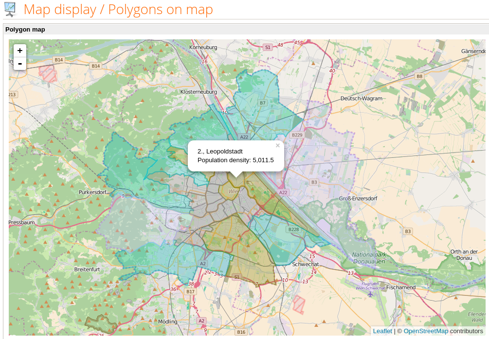
Als zusätzliche Information erzeugen wir mit .bindPopup(...) noch ein Popup-Fenster, das beim Klick auf einen Bezirk angezeigt wird und zusätzliche Informationen enthält.
Linien-Daten werden ganz ähnlich angezeigt und verarbeitet. Bei Punkt-Daten können verschiedene Marker definiert werden, bei Leaflet gibt es die Anleitung dazu.
Damit ist das Ziel erreicht: RapidMiner Server zeigt eine Karte an, deren Daten (Punkte, Linien oder Flächen) in einen RapidMiner-Prozess verarbeitet wurden.
Displaying geographic data in RapidMiner Server
Update 2020-02: GIS functionality is now available in an extension.
After the series of blog posts about GIS in RapidMiner Studio (1, 2, 3, 4) we’d probably like to visualize our results. The mechanisms in Studio are quite limited: we can create scatter plots from point data but there is no good method for displaying lines and areas.
However, RapidMiner Server offers webapps and powerful visualization using JavaScript.
Using GeoScript in processes
For displaying geographic data it’s not necessary to set up the server with the GeoScript libraries. However, if you want to execute the GIS processes like in studio, it can be a good idea to do so.
Start with the geoscript directory set up in the first part. You’ll need a Zip utility; I used Midnight Commander.
- Stop RapidMiner Server
- Make a backup copy of rapidminer-server/standalone/deployments/rapidminer-server-X.Y.Z.ear somewhere else
- Delete the old groovy-X.jar from the lib/ directory and put in the new one from the Studio installation
- Copy all jar files from the geoscript directory of the Studio installation to lib/. Existing files don’t need to be overwritten.
- Start RapidMiner Server.
After this process, all your Studio GIS processes should work in the Server.
Map display in webapps
I chose the Leaflet library, as it is open source and well documented. There is no special GIS data type in RapidMiner and the processes in the tutorials used WKT (Well Known Text) until now, so we’ll also need the Mapbox Omnivore library. This converts WKT data to GeoJSON which Leaflet prefers.
Before starting with the web app, we need to build a process in Studio for creating the data. An example process could use the district boundaries as CSV and the population statistics from the Vienna Open Data server. It joins the districts using a common attribute (NUTS id). The output of the process is a table with the district boundaries, their area, the total population and the population density. We also use Generate Attributes to classify the population density with HTML colors (#AABBCC notation). You can get creative here and use the entire functionality of RapidMiner.
The process is saved on the server. We create a new entry in Processes/Services and call it for example ViennaDistrictPopDensitySvc. The data source is the process created before, the output format is JSON. It is a good idea to set up this web service for public anonymous access.
In a new web app we create a Text component and uncheck the „Use graphical editor“ checkbox to enter HTML and JavaScript code.
Infrastructure
<div id="map">
</div>

<script type="text/javascript" src="http://cdn.leafletjs.com/leaflet-0.6.4/leaflet.js"></script>
<link rel="stylesheet" type="text/css" href="http://cdn.leafletjs.com/leaflet-0.6.4/leaflet.css"/>
<script src="https://api.mapbox.com/mapbox.js/plugins/leaflet-omnivore/v0.2.0/leaflet-omnivore.min.js"></script>

<style type="text/css">
#map {
    height: 650px;
}
</style>
This part fetches the Leaflet and Omnivore components and creates a DIV object for the map. We specify the map height in pixels in the CSS block (e. g. 650px).
Then a JavaScript block is started with <script language="JavaScript">. Don’t forget to close the block with </script> at the end.
Setting up the base map
// Create the map
var map = L.map('map').setView([48.17, 16.4], 11);
// Set up the OSM layer
L.tileLayer(
'http://{s}.tile.openstreetmap.org/{z}/{x}/{y}.png',
{
maxZoom: 18,
attribution: '© <a href="http://osm.org/copyright">OpenStreetMap</a> contributors; District data: Open Data Vienna'
}
).addTo(map);
This creates a map object with an OpenStreetMap background layer. The initialization parameters are latitude and longitude of the initial position, and the zoom level (11 in this example).
There are many tile servers available. Be sure to check the terms of usage and update the attribution appropriately.
Getting data from the RapidMiner process
var Httpreq = new XMLHttpRequest();
Httpreq.open("GET","/api/rest/public/process/ViennaDistrictPopDensitySvc?",false);
Httpreq.send(null);
var mapdata = JSON.parse(Httpreq.responseText);
This part fetches the data in JSON format from the local RapidMiner Server and stores them in the mapdata variable. To refer to another web service, change the URL.
Displaying the objects on the map
for (i = 0; i < mapdata.length; i++) {
  var district = omnivore.wkt.parse(mapdata[i].SHAPE);
  district.addTo(map)
    .bindPopup(mapdata[i].NAME + "
Population density: " + mapdata[i].POP_DENSITY)
    .setStyle({color: mapdata[i].densityColor, weight: 2, fillOpacity: 0.3});
}
Here, a loop processes the process results. The Omnivore function converts the district area (SHAPE attribute in the example data) to a new object on the map.
We assign the color calculated in the process with .setStyle(...) (densityColor attribute in this example).
We also create a popup window with additional information using .bindPopup(...). It will be displayed when the user clicks a district.
Displaying line data is very similar. For displaying point data, you can use different markers. This is described by a Leaflet tutorial.
So we reached our goal: RapidMiner Server displays a map with data (points, lines or areas or even a combination) coming from a RapidMiner process.