Schlagwort-Archive: JSON

JSON-Verarbeitung mit Jq

(English version)

jq ist ein Werkzeug zur Verarbeitung von JSON-Dokumenten. Es bietet Filter, Umformungen, Umstrukturierungen und andere Möglichkeiten, um die Dokumente in die gewünschte Form zu bringen.

Die JSON-Dokumente, mit denen man als Data Scientist zu tun hat, werden immer komplexer. Z. B. kommt von einer Web-API ein Dokument, das hierarchische, optionale Elemente enthält.

Für Data Mining braucht man jedoch immer eine tabellarische Struktur, ohne hierarchische Elemente und idealerweise auch ohne fehlende Daten. jq hilft dabei, die relevanten Teile der Eingangsdokumente in so eine Form zu bringen.

Nehmen wir folgendes simples Beispieldokument:

{
    "count": 3,
    "category": "example",
    "elements": [
        {
            "id": 1,
            "description": "first element",
            "tags": ["tag1"]
        },
        {
            "id": 2,
            "description": "second element",
            "optional": "optional element",
            "tags": []
        },
        {
            "id": 3,
            "description": "third element",
            "tags": ["tag1", "tag2"]
        }
    ]
}

Wir sehen hier die üblichen Fallstricke komplexer JSON-Dokumente:

  • Elemente auf unterschiedlichen Hierarchiestufen: category, elements/id usw.
  • Optionale Elemente: elements[2]/optional
  • Variable Anzahl von Elementen: elements/tags

jq bietet eine relativ einfache Syntax, um solche Konstrukte zu verarbeiten. Am einfachsten ist es, die Ausdrücke online bei jqplay.org zu entwickeln.

Vielleicht ist das Ziel, eine Tabelle mit category, der Element-Id und den Tags zu erstellen. Der jq-Ausdruck dafür lautet:

{count, category, elements: .elements[] } | {category, id: .elements.id, tag: .elements.tags[]}

Auf den ersten Blick etwas furchteinflößend, aber letztendlich aus einfachen Elementen aufgebaut. Wenn man den Ausdruck Schritt für Schritt bei jqplay ausführt, wird es klarer.

Im ersten Schritt (die Schritte sind mit dem Pipe-Symbol | getrennt) deklarieren wir, welche Elemente wir verarbeiten möchten. Dabei wird eine Liste von Objekten mit {} aufgebaut, darin count und category aus der Hauptebene des Dokuments, und die Elemente als Array. count und category werden dabei wiederholt, damit die „Tabelle“ vollständig ist.

Im zweiten Schritt selektieren wir die category (ursprünglich auf der Hauptebene) und die id jedes Objekts; dazu die Tags als Array. Mit name: .hauptelement.kindelement können wir Elemente selektieren und benennen. Das Ergebnis dieses Schrittes ist eine Liste von Objekten mit category, id, und tag in einer tabellarischen Struktur, die wir etwa in eine Datenbank schreiben oder in einem Data-Mining-Tool verarbeiten könnten.

jq in RapidMiner

Um so komplexe Dokumente in RapidMiner verarbeiten zu können, wäre es praktisch, jq direkt einzubinden. Genau das habe ich gemacht, mit Hilfe von jackson-jq, einer Java-Implementierung.

Zur Vorbereitung müssen wir die Jar-Datei von jackson-jq und zwei Abhängigkeiten ins lib-Verzeichnis von RapidMiner Studio kopieren. Danach steht die Funktionalität im eingebauten Groovy Scripting Operator (Execute Script) zur Verfügung.

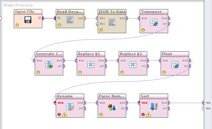
Um die Anwendung zu vereinfachen, habe ich zwei RapidMiner-Prozesse erstellt, die in eigenen Prozessen eingebunden werden können. Eine Variante arbeitet an Tabellen (Example Sets), hier muß man beim Aufruf festlegen, welches Attribut die Eingangsdaten enthält und wie das Zielattribut mit dem Ergebnis der Transformation heißen soll. Die andere Variante arbeitet an Document-Objekten, wie sie etwa von Get Page geliefert werden.

In beiden Fällen kann man noch den jq-Ausdruck angeben, festlegen, ob der Output eingerückt formatiert werden soll, und letztendlich wählen, ob das Ergebnis in CSV konvertiert werden soll. Das CSV-formatierte Ergebnis kann RapidMiner mit Read CSV sehr einfach in eine Tabelle umwandeln — das ist bei mir häufig das Ziel.

In jqplay würden wir für den CSV-Output noch folgendes anhängen, und „Raw Output“ auswählen:

 | [ .category, .id, .tag ] | @csv

Damit erzeugen wir ein Array (mit der []-Syntax) und nennen die auszugebenden Elemente. Das Ergebnis wird dann mit @csv umformatiert. (Diesen letzten Schritt erledigt der RapidMiner-Prozess automatisch, wenn der CSV-Output ausgewählt ist.)

Mit etwas Üben und der Hilfe von jqplay lassen sich somit Prozesse erstellen, die aus einem verschachtelten JSON-Dokument relativ einfach eine gut handhabbare Tabelle erstellen.

Um verschiedene Hierarchien innerhalb des Dokuments zu verarbeiten, könnte man auch verschiedene jq-Ausdrücke anwenden, und daraus unterschiedliche Tabellen erhalten.

Processing JSON with jq

jq is a command line tool for processing JSON documents. It can filter, transform and restructure documents to format them in the way we want.

The JSON documents data scientists have to work with are becoming more and more complex. Web APIs often generate documents with hierarchic structure and optional elements.

Data mining, however, needs a tabular structure, without hierarchic elements, and if possible without missing data. jq helps us with the transformation of relevant parts of input documents into this shape.

Take the following example document:

{
    "count": 3,
    "category": "example",
    "elements": [
        {
            "id": 1,
            "description": "first element",
            "tags": ["tag1"]
        },
        {
            "id": 2,
            "description": "second element",
            "optional": "optional element",
            "tags": []
        },
        {
            "id": 3,
            "description": "third element",
            "tags": ["tag1", "tag2"]
        }
    ]
}

This shows the usual pitfalls of complex JSON documents:

  • Elements on different hierarchy levels: category, elements/id etc.
  • Optional elements: elements[2]/optional
  • Variable number of elements: elements/tags

The easiest way to try jq is online at jqplay.org.

We might want to create a table with the category, the element id and the tags. The jq expression for this is:

{count, category, elements: .elements[] } | {category, id: .elements.id, tag: .elements.tags[]}

Scary for sure in the first moment! But when you look at it, it’s built of simple elements. You can always execute it step by step at jqplay to see the effects of each step.

In the first step (the steps being delimited by the pipe symbol „|“) we declare the elements we want to process. We build an object list with { }, taking count and category from the top level and an array of the elements. count and category are repeated to create a proper table.

In the second step we select category and the object id-s, which were on different levels previously. The tags are selected as an array. Using the syntax name: .element.element we can select elements and name them. The result of this step is a list of objects having category, id and tag in a table, suitable for writing into a relational database or processing in a data mining tool.

jq in RapidMiner

It would be useful to process these kinds of documents with jq in RapidMiner. This is what I did, using jackson-jq, a Java implementation of jq.

To prepare, we need to copy the jackson-jq jar file and two dependencies into the RapidMiner Studio lib directory. Then we’re able to use the functionality in the built-in Groovy scripting operator (Execute Script).

I created two RapidMiner processes to make the application easier. These can be used in other processes. There is one variant working on tables (example sets), here you specify the name of the input attribute containing your documents and the target attribute for the transformation result. The other variant works on Document objects, like those coming from Get Page.

In both cases you specify the jq expression and set up the output options. You can indent the output, and convert the result to CSV. The CSV formatted result can be easily transformed to an example set — this is a frequent use case.

If you want to see CSV output in jqplay, check „Raw Output“ and append the following:

 | [ .category, .id, .tag ] | @csv

This creates an array (with the [] syntax) and lists the elements in the output. The result is converted with the @csv step. (The RapidMiner process does this automatically if the csv output is selected.)

This, together with some practicing in jqplay, enables processes that can transform complex JSON documents to straight tables.

To process different parts and structures in the document, just multiply it and apply different jq expressions on the copies.

Visualisierung von Geodaten in RapidMiner Server

(English version)

Update 2020-02: GIS-Funktionalität ist jetzt als Erweiterung verfügbar.

Nach der Artikelserie über GIS in RapidMiner Studio (1234) geht es nun darum, wie die erhaltenen Ergebnisse visualisiert werden können. In Studio sind die Möglichkeiten dafür ja ziemlich eingeschränkt: Punkt-Daten können noch halbwegs als Scatterplots angezeigt werden, aber für Linien und Flächen gibt es keine guten Methoden.

RapidMiner Server bietet aber mit den Webapps die Möglichkeit einer flexiblen Visualisierung durch die Einbindung von JavaScript.

Einbindung von GeoTools

Für die nachfolgende Vorgehensweise ist es nicht notwendig, den Server ähnlich wie Studio mit Geo-Libraries auszustatten. Wenn man jedoch die gleichen GIS-Funktionen wie in Studio verwenden will, kann es sinnvoll sein.

Ausgehend vom eingerichteten geoscript-Verzeichnis wie im ersten Teil der Anleitung werden die Jar-Bibliotheken aus diesem Verzeichnis in die EAR-Datei des Servers kopiert. Man braucht dazu ein Zip-Werkzeug, ich habe den Midnight Commander verwendet.

  1. RapidMiner Server beenden
  2. rapidminer-server/standalone/deployments/rapidminer-server-X.Y.Z.ear zur Sicherheit anderswo hinkopieren
  3. Aus dem lib/-Verzeichnis die alte groovy-X.jar löschen und die neue aus der Studio-Installation hineinkopieren
  4. Alle Jar-Dateien aus dem geoscript-Ordner der Studio-Installation auch in lib/ kopieren. Wenn eine Datei schon vorhanden ist, muß sie nicht überschrieben werden.
  5. RapidMiner Server starten.

Danach sollten alle Prozesse mit GIS-Verarbeitung aus Studio auch am Server funktionieren.

Visualisierung in Webapps

Meine Wahl fiel auf die Leaflet-Library, da sie Open Source und gut dokumentiert ist. Da wir in RapidMiner keinen eigenen GIS-Datentyp haben und die bisherigen Prozesse die Geodaten als WKT (Well Known Text)  verarbeiten, brauchen wir noch die Mapbox-Omnivore-Library. Diese konvertiert WKT-Daten in GeoJSON, das bevorzugte Format von Leaflet.

Vor der Erstellung des Webapps bauen wir einen Prozess in Studio, der die gewünschten Daten ausgibt. Ein Beispielprozess könnte vom Wiener Open-Data-Server die Bezirksgrenzen als CSV und Bevölkerungsstatistiken holen. Die Bezirke werden über ein gemeinsames Feld (NUTS-Id) verknüpft. Der Output des Prozesses ist eine Tabelle mit den Geodaten des Bezirks, ihrer Fläche, der Gesamtbevölkerung und der Bevölkerungsdichte. Für die Bevölkerungsdichte errechnen wir mit Generate Attributes die Anzahl der Personen pro Quadratkilometer und klassifizieren sie, indem wir verschiedenen Wertbereichen HTML-Farben in der #AABBCC-Notation zuweisen. Hier ist die eigene Kreativität gefragt.

Der Prozess wird auf den Server gelegt. Unter Processes/Services legen wir eine neue Eintragung an und nennen sie z. B. ViennaDistrictPopDensitySvc. Wir wählen als Datenquelle den vorhin angelegten Prozess und als Output Format JSON. Es ist sinnvoll, dieses Webservice als anonym/öffentlich aufzusetzen, um zusätzliche Paßworteingaben zu vermeiden.

In der neuen Webapplikation erzeugen wir eine Komponente vom Typ Text, und schalten „Use graphical editor“ ab. Danach geben wir den HTML- und JavaScript-Code ein.

Infrastruktur

<div id="map">
</div>

<script type="text/javascript" src="http://cdn.leafletjs.com/leaflet-0.6.4/leaflet.js"></script>
<link rel="stylesheet" type="text/css" href="http://cdn.leafletjs.com/leaflet-0.6.4/leaflet.css"/>
<script src="https://api.mapbox.com/mapbox.js/plugins/leaflet-omnivore/v0.2.0/leaflet-omnivore.min.js"></script>

<style type="text/css">
 #map {
 height: 650px;
}
</style>

Dieser Teil holt die Leaflet- und Omnivore-Komponenten und erzeugt ein Objekt, in das die Karte eingefügt werden kann. Im CSS wird die Höhe in Pixeln angegeben (z. B. 650px).

Danach starten wir mit <script language="JavaScript"> einen JavaScript-Block, der am Ende mit </script> geschlossen wird.

Definition der Basiskarte

// Create the map
var map = L.map('map').setView([48.17, 16.4], 11);
// Set up the OSM layer
L.tileLayer(
    'http://{s}.tile.openstreetmap.org/{z}/{x}/{y}.png',
    {
       maxZoom: 18,
       attribution: '&copy; <a href="http://osm.org/copyright">OpenStreetMap</a> contributors; District data: Open Data Vienna'
    }
).addTo(map);

Hier erzeugen wir das Kartenobjekt mit einer OpenStreetMap-Hintergrundkarte. Die Initialisierungsparameter sind Längen- und Breitengrad der anfänglichen Position der Karte, die Zahl dahinter (11 in diesem Beispiel) die Zoom-Stufe.

Es gibt viele Tile-Server, man sollte die Nutzungsbedingungen prüfen und die Herkunftsangabe (attribution) entsprechend anpassen.

Daten des RapidMiner-Prozesses holen

var Httpreq = new XMLHttpRequest();
Httpreq.open("GET","/api/rest/public/process/ViennaDistrictPopDensitySvc?",false);
Httpreq.send(null);
var mapdata = JSON.parse(Httpreq.responseText);

Dieser Block holt vom lokalen (oder auch einem beliebigen anderen) RapidMiner Server die Daten des Prozesses im JSON-Format und legt sie im mapdata-Objekt ab. Die URL des Webservice kann hier angepaßt werden.

Anzeige der Geo-Objekte

for (i = 0; i < mapdata.length; i++) {
  var district = omnivore.wkt.parse(mapdata[i].SHAPE);
  district.addTo(map)
    .bindPopup(mapdata[i].NAME + "
Population density: " + mapdata[i].POP_DENSITY)
    .setStyle({color: mapdata[i].densityColor, weight: 2, fillOpacity: 0.3});
}

Hier verarbeiten wir die Ergebnisse des Prozesses in einer Schleife. Aus jeder Zeile wird die Form des Bezirks (Attribut SHAPE in den Beispieldaten) mit Hilfe von Omnivore konvertiert, und als neues Objekt zur Karte hinzugefügt.
Mit .setStyle(...) ordnen wir die im Prozess erzeugte Farbabstufung (im Beispiel das densityColor-Attribut) zu.
Als zusätzliche Information erzeugen wir mit .bindPopup(...) noch ein Popup-Fenster, das beim Klick auf einen Bezirk angezeigt wird und zusätzliche Informationen enthält.

Linien-Daten werden ganz ähnlich angezeigt und verarbeitet. Bei Punkt-Daten können verschiedene Marker definiert werden, bei Leaflet gibt es die Anleitung dazu.

Damit ist das Ziel erreicht: RapidMiner Server zeigt eine Karte an, deren Daten (Punkte, Linien oder Flächen) in einen RapidMiner-Prozess verarbeitet wurden.

Bevölkerungsdichte pro Bezirk in Wien
Bevölkerungsdichte pro Bezirk in Wien (Daten: Open Data Wien)

Displaying geographic data in RapidMiner Server

Update 2020-02: GIS functionality is now available in an extension.

After the series of blog posts about GIS in RapidMiner Studio (1234) we’d probably like to visualize our results. The mechanisms in Studio are quite limited: we can create scatter plots from point data but there is no good method for displaying lines and areas.

However, RapidMiner Server offers webapps and powerful visualization using JavaScript.

Using GeoScript in processes

For displaying geographic data it’s not necessary to set up the server with the GeoScript libraries. However, if you want to execute the GIS processes like in studio, it can be a good idea to do so.

Start with the geoscript directory set up in the first part. You’ll need a Zip utility; I used Midnight Commander.

  1. Stop RapidMiner Server
  2. Make a backup copy of rapidminer-server/standalone/deployments/rapidminer-server-X.Y.Z.ear somewhere else
  3. Delete the old groovy-X.jar from the lib/ directory and put in the new one from the Studio installation
  4. Copy all jar files from the geoscript directory of the Studio installation to lib/. Existing files don’t need to be overwritten.
  5. Start RapidMiner Server.

After this process, all your Studio GIS processes should work in the Server.

Map display in webapps

I chose the Leaflet library, as it is open source and well documented. There is no special GIS data type in RapidMiner and the processes in the tutorials used WKT (Well Known Text) until now, so we’ll also need the Mapbox Omnivore library. This converts WKT data to GeoJSON which Leaflet prefers.

Before starting with the web app, we need to build a process in Studio for creating the data. An example process could use the district boundaries as CSV and the population statistics from the Vienna Open Data server. It joins the districts using a common attribute (NUTS id). The output of the process is a table with the district boundaries, their area, the total population and the population density. We also use Generate Attributes to classify the population density with HTML colors (#AABBCC notation). You can get creative here and use the entire functionality of RapidMiner.

The process is saved on the server. We create a new entry in Processes/Services and call it for example ViennaDistrictPopDensitySvc. The data source is the process created before, the output format is JSON. It is a good idea to set up this web service for public anonymous access.

In a new web app we create a Text component and uncheck the „Use graphical editor“ checkbox to enter HTML and JavaScript code.

Infrastructure

<div id="map">
</div>

<script type="text/javascript" src="http://cdn.leafletjs.com/leaflet-0.6.4/leaflet.js"></script>
<link rel="stylesheet" type="text/css" href="http://cdn.leafletjs.com/leaflet-0.6.4/leaflet.css"/>
<script src="https://api.mapbox.com/mapbox.js/plugins/leaflet-omnivore/v0.2.0/leaflet-omnivore.min.js"></script>

<style type="text/css">
#map {
    height: 650px;
}
</style>

This part fetches the Leaflet and Omnivore components and creates a DIV object for the map. We specify the map height in pixels in the CSS block (e. g. 650px).

Then a JavaScript block is started with <script language="JavaScript">. Don’t forget to close the block with </script> at the end.

Setting up the base map

// Create the map
var map = L.map('map').setView([48.17, 16.4], 11);
// Set up the OSM layer
L.tileLayer(
    'http://{s}.tile.openstreetmap.org/{z}/{x}/{y}.png',
    {
       maxZoom: 18,
       attribution: '&copy; <a href="http://osm.org/copyright">OpenStreetMap</a> contributors; District data: Open Data Vienna'
    }
).addTo(map);

This creates a map object with an OpenStreetMap background layer. The initialization parameters are latitude and longitude of the initial position, and the zoom level (11 in this example).

There are many tile servers available. Be sure to check the terms of usage and update the attribution appropriately.

Getting data from the RapidMiner process

var Httpreq = new XMLHttpRequest();
Httpreq.open("GET","/api/rest/public/process/ViennaDistrictPopDensitySvc?",false);
Httpreq.send(null);
var mapdata = JSON.parse(Httpreq.responseText);

This part fetches the data in JSON format from the local RapidMiner Server and stores them in the mapdata variable. To refer to another web service, change the URL.

Displaying the objects on the map

for (i = 0; i < mapdata.length; i++) {
  var district = omnivore.wkt.parse(mapdata[i].SHAPE);
  district.addTo(map)
    .bindPopup(mapdata[i].NAME + "
Population density: " + mapdata[i].POP_DENSITY)
    .setStyle({color: mapdata[i].densityColor, weight: 2, fillOpacity: 0.3});
}

Here, a loop processes the process results. The Omnivore function converts the district area (SHAPE attribute in the example data) to a new object on the map.
We assign the color calculated in the process with .setStyle(...) (densityColor attribute in this example).
We also create a popup window with additional information using .bindPopup(...). It will be displayed when the user clicks a district.

Displaying line data is very similar. For displaying point data, you can use different markers. This is described by a Leaflet tutorial.

So we reached our goal: RapidMiner Server displays a map with data (points, lines or areas or even a combination) coming from a RapidMiner process.

Population density by district in Vienna
Population density by district in Vienna (Data: Open Data Vienna)

JSON-Verarbeitung in RapidMiner

(English version below)

Da man immer wieder auf Datenquellen im JSON-Format stößt, möchte ich auch zeigen, wie man sie mit RapidMiner verarbeitet.

Früher gab es nur den Operator „Json to XML“. Dieser versucht, die JSON-Datenstruktur in XML abzubilden, sodaß man sie dann mit dem vorhandenen Read XML-Operator verarbeiten kann. Leider schlägt das in vielen Fällen fehl, da JSON wesentlich weniger strukturiert sein kann als XML.

Mit der Version 6.2 wurde aber ein genialer Operator eingeführt, der die Verarbeitung extrem erleichtert und elegant macht: Json to Data. Im Prinzip bildet er die Struktur des JSON-Dokuments mit der kompletten Hierarchie inkl. Arrays in Spalten ab, die nach dem „JSON-Pfad“ zum Element benannt sind.

Natürlich können da sehr breite Datenstrukturen rauskommen, aber damit hat RapidMiner kein Problem. Mit einem simplen Trick kann man diese „unbequeme“ Datenstruktur bearbeiten: Der Transpose-Operator transponiert die Spalten in Zeilen, und erzeugt damit eine viel simplere Tabelle, die leicht weiterzuverarbeiten ist.

So sieht der Prozess zur Verarbeitung des JSON-Dokuments aus dem letzten Betrag aus:

RapidMiner-Prozess zur JSON-Verarbeitung

(Prozess herunterladen)

Open File öffnet die URL und gibt ein File-Objekt aus. Read Document liest den Inhalt des File-Objekts und gibt ihn als Document (unstrukturierter Text) aus. JSON To Data konvertiert das Dokument in eine RapidMiner-Tabelle (in diesem Fall mit 24.000 Spalten und einer Zeile). Transpose klappt die Zeilen und Spalten dann um.

Es ist sinnvoll, einen Haltepunkt auf Transpose zu setzen (F7, Breakpoint after) und die Daten anzuschauen. Es gibt eine ID-Spalte, die den Pfad zu den Daten (in diesem Fall in Array-Syntax: [x][y]) enthält, und eine Attribut-Spalte, die die Daten selbst enthält. Alles wurde in Strings konvertiert.

Beispiel-Ausgabe:

id att_1
[0][0] 194.0
[0][10] Conglomerates
[0][11] Minnesota

Da wir die zwei Dimensionen des Arrays in zwei separaten Spalten brauchen, kopieren wir die ID-Spalte, und transformieren sie und ihre Kopie mit regulären Ausdrücken. Das Ergebnis sieht so aus:

id id2 att_1
0 0 194.0
0 10 Conglomerates
0 11 Minnesota

Das id-Feld ist die Gruppe und das id2-Feld der Spaltenindex. Diese Struktur wird mit dem Pivot-Operator so konvertiert, daß id die Zeile definiert und id2 die Spalten. Diese brauchen dann nur mehr umbenannt zu werden. Danach werden noch die String-Spalten in Zahlen konvertiert und das Ergebnis nach dem Sort-Feld sortiert.

Fertig! Elegant und intuitiv, wie von RapidMiner gewohnt.

Processing JSON documents in RapidMiner

Data scientists frequently have the requirement to process JSON documents. I’d like to show how one can process them in RapidMiner.

Until recently, the only way was using the operator „Json to XML“. This operator tries to convert the original structure of the JSON document to XML so it can be processed using Read XML. Unfortunately, JSON is usually less structured than XML so this fails quite often.

A great operator was introduced in  version 6.2 that makes processing JSON much easier and more elegant: Json to Data. It converts the structure of the JSON document to columns named by the „JSON path“ of the element.

This can lead to very broad data structures with hundreds or thousands of columns, but this is not a problem for RapidMiner. Using a simple trick, this unusual data representation can be changed: the Transpose operator flips columns to rows, so the table becomes much simpler.

This is a process for loading an example JSON array from the web and converting it into a tabular structure with metadata:

RapidMiner process for processing JSON

(Download process)

Open File loads the contents from the URL and returns a File object. Read Document reads the contents of the file and returns an unstructured Document object. JSON to Data takes the document and converts it into a RapidMiner example set. (In this case, the table has 24,000 columns and one row.) Transpose changes the columns into rows.

You could set a breakpoint on Transpose (F7, Breakpoint after) and look at the data. There’s an ID column which contains the JSON path of the attribute value (in this case, in array syntax: [x][y]), and an attribute value column with the data. Everything was converted to strings.

Example:

id att_1
[0][0] 194.0
[0][10] Conglomerates
[0][11] Minnesota

We need both dimensions of the array as separate columns, so we copy the ID column and transform both copies using regular expressions. This is the result:

id id2 att_1
0 0 194.0
0 10 Conglomerates
0 11 Minnesota

The id field is the group and id2 the column index. This structure is processed with the Pivot operator by using id as the row identifier and id2 as the column. Then we rename the columns, convert string columns to numbers and sort the results by the value of the Sort field.

That’s it! Elegant and intuitive, thanks to RapidMiner.

JSON-Array in PostgreSQL verarbeiten

(English version)

Neulich mußte ich eine JSON-Datenstruktur aus einer Web-Quelle holen und in die Datenbank einfügen. Das Besondere an diesen Daten ist, daß sie einfach in einem zweidimensionalen Array liegen, die Webseite interpretiert die Daten selbst. Es sind also keine Feldnamen im JSON.

In R ging es recht einfach:

require(rjson)

# JSON-Array laden, List daraus machen
global2k_lst <- fromJSON(file="http://www.forbes.com/ajax/load_list/?type=organization&uri=global2000&year=2014");
# Die Liste in einen eindimensionalen Vektor konvertieren
global2k <- unlist(global2k_lst)
# Durch die Angabe der Dimensionen wird eine Matrix daraus
dim(global2k) <- c(12,2000)
# Aus der Matrix dann ein Data Frame machen und die Felder benennen
global2k <- as.data.frame(t(global2k))
names(global2k) <- c("rank", "urlname", "name", "logoname", "sort",
                     "sales", "profits", "assets", "marketvalue",
                     "country", "industry", "us_state")

write.csv2(global2k, "/tmp/forbes2000.csv", row.names=FALSE)

Andererseits hat PostgreSQL seit Version 9.3 viele JSON-Funktionen. Wie funktioniert es also direkt in der Datenbank?

Erst mal habe ich den ganzen JSON-String in eine Tabelle ins Feld „forbes2k_json“ eingelesen. (PostgreSQL hat ja auch mit 244 kByte Daten in einem Feld kein Problem.) Der Inhalt des Arrays läßt sich dann mit PostgreSQL-Mitteln mit etwas Aufwand als Tabelle ausgeben:

-- JSON-Array in 2000 Zeilen aufspalten
with lines as (
    select json_array_elements(forbes2k_json::json) as company
    from forbes2k_json
),
-- Die Elemente der Zeilen in jeweils 12 Zeilen aufspalten, die Original-Zeilen nummerieren
entries as (
    select json_array_elements(company)::text as entry,
        row_number() over () as entrynr
    from lines
),
-- Die Felder nummerieren
fields as (
    select *,
        row_number() over (partition by entrynr) as fieldnr
    from entries
)
-- Mit 12 self joins die Tabellenstruktur aufbauen und die Felder konvertieren
select f1.entry::integer as rank,
    regexp_replace(f2.entry::text, '^"(.*)"$', '\1') as urlname,
    regexp_replace(f3.entry::text, '^"(.*)"$', '\1') as company,
    regexp_replace(f4.entry::text, '^"(.*)"$', '\1') as logoname,
    f5.entry::integer as sort,
    regexp_replace(regexp_replace(f6.entry::text, ',', ''), '^"(.*)"$', '\1')::numeric(10,3) as sales,
    regexp_replace(regexp_replace(f7.entry::text, ',', ''), '^"(.*)"$', '\1')::numeric(10,3) as profits,
    regexp_replace(regexp_replace(f8.entry::text, ',', ''), '^"(.*)"$', '\1')::numeric(10,3) as assets,
    regexp_replace(regexp_replace(f9.entry::text, ',', ''), '^"(.*)"$', '\1')::numeric(10,3) as marketvalue,
    regexp_replace(f10.entry::text, '^"(.*)"$', '\1') as country,
    regexp_replace(f11.entry::text, '^"(.*)"$', '\1') as industry,
    regexp_replace(f12.entry::text, '^"(.*)"$', '\1') as us_state
from fields f1
inner join fields f2 on f2.entrynr = f1.entrynr and f2.fieldnr = 2
inner join fields f3 on f3.entrynr = f1.entrynr and f3.fieldnr = 3
inner join fields f4 on f4.entrynr = f1.entrynr and f4.fieldnr = 4
inner join fields f5 on f5.entrynr = f1.entrynr and f5.fieldnr = 5
inner join fields f6 on f6.entrynr = f1.entrynr and f6.fieldnr = 6
inner join fields f7 on f7.entrynr = f1.entrynr and f7.fieldnr = 7
inner join fields f8 on f8.entrynr = f1.entrynr and f8.fieldnr = 8
inner join fields f9 on f9.entrynr = f1.entrynr and f9.fieldnr = 9
inner join fields f10 on f10.entrynr = f1.entrynr and f10.fieldnr = 10
inner join fields f11 on f11.entrynr = f1.entrynr and f11.fieldnr = 11
inner join fields f12 on f12.entrynr = f1.entrynr and f12.fieldnr = 12
where f1.fieldnr = 1
order by rank, sort

Kompliziert ist es nicht, nur viel zu tippen (und copy/paste-en). Da die Daten selbst keine Feld-Metadaten wie Name und Typ enthalten, muß man sie selbst festlegen.

Processing a JSON array in PostgreSQL

I needed to get a JSON data structure from the web and put its contents into a database. These data were a bit special in the sense that the JSON only contained only a two dimensional array interpreted by the website, without any field names.

In R it was quite easy:

require(rjson)

# Load JSON array and convert to a list
global2k_lst <- fromJSON(file="http://www.forbes.com/ajax/load_list/?type=organization&uri=global2000&year=2014");
# Convert to a one-dimensional vector
global2k <- unlist(global2k_lst)
# Change to a matrix by specifying the dimensions
dim(global2k) <- c(12,2000)
# Convert the matrix to a data frame and specify the field names
global2k <- as.data.frame(t(global2k))
names(global2k) <- c("rank", "urlname", "name", "logoname", "sort",
                     "sales", "profits", "assets", "marketvalue",
                     "country", "industry", "us_state")

write.csv2(global2k, "/tmp/forbes2000.csv", row.names=FALSE)

On the other hand, PostgreSQL has lots of JSON functions since release 9.3. So how to do it directly in the database?

The first step is reading the entire JSON string into a table in a field called „forbes2k_json“. (PostgreSQL can easily store 244 kBytes of data in a single field.) A not too complex query converts the array contents into a normal table:

-- JSON array into 2000 lines
with lines as (
    select json_array_elements(forbes2k_json::json) as company
    from forbes2k_json
),
-- Existing lines converted into 12 lines each, with an additional row number for 
-- the original lines
entries as (
    select json_array_elements(company)::text as entry,
        row_number() over () as entrynr
    from lines
),
-- Row numbers of the entry lines
fields as (
    select *,
        row_number() over (partition by entrynr) as fieldnr
    from entries
)
-- 12 self joins for building the table structure; convert field types
select f1.entry::integer as rank,
    regexp_replace(f2.entry::text, '^"(.*)"$', '\1') as urlname,
    regexp_replace(f3.entry::text, '^"(.*)"$', '\1') as company,
    regexp_replace(f4.entry::text, '^"(.*)"$', '\1') as logoname,
    f5.entry::integer as sort,
    regexp_replace(regexp_replace(f6.entry::text, ',', ''), '^"(.*)"$', '\1')::numeric(10,3) as sales,
    regexp_replace(regexp_replace(f7.entry::text, ',', ''), '^"(.*)"$', '\1')::numeric(10,3) as profits,
    regexp_replace(regexp_replace(f8.entry::text, ',', ''), '^"(.*)"$', '\1')::numeric(10,3) as assets,
    regexp_replace(regexp_replace(f9.entry::text, ',', ''), '^"(.*)"$', '\1')::numeric(10,3) as marketvalue,
    regexp_replace(f10.entry::text, '^"(.*)"$', '\1') as country,
    regexp_replace(f11.entry::text, '^"(.*)"$', '\1') as industry,
    regexp_replace(f12.entry::text, '^"(.*)"$', '\1') as us_state
from fields f1
inner join fields f2 on f2.entrynr = f1.entrynr and f2.fieldnr = 2
inner join fields f3 on f3.entrynr = f1.entrynr and f3.fieldnr = 3
inner join fields f4 on f4.entrynr = f1.entrynr and f4.fieldnr = 4
inner join fields f5 on f5.entrynr = f1.entrynr and f5.fieldnr = 5
inner join fields f6 on f6.entrynr = f1.entrynr and f6.fieldnr = 6
inner join fields f7 on f7.entrynr = f1.entrynr and f7.fieldnr = 7
inner join fields f8 on f8.entrynr = f1.entrynr and f8.fieldnr = 8
inner join fields f9 on f9.entrynr = f1.entrynr and f9.fieldnr = 9
inner join fields f10 on f10.entrynr = f1.entrynr and f10.fieldnr = 10
inner join fields f11 on f11.entrynr = f1.entrynr and f11.fieldnr = 11
inner join fields f12 on f12.entrynr = f1.entrynr and f12.fieldnr = 12
where f1.fieldnr = 1
order by rank, sort